Reinforcement Learning for Dynamic Wealth Optimization and Asset-Liability Management

Detailed Report

Introduction to Lifetime Portfolio Optimization

The allocation of capital over a human lifecycle represents a foundational problem in quantitative economics, originally formalized by Robert Merton in 1969. In its purest form, the Merton portfolio problem seeks to find the mathematical policy where an individual or institutional asset manager continuously divides wealth between risky and risk-free assets to maximize expected lifetime utility.

However, a steep divergence occurs between textbook economic abstractions and empirical reality. Traditional models assume smooth, continuous transitions. Real life is inherently discontinuous. For an institutional pension fund or an individual investor, wealth trajectories are continually disrupted by non-linear shocks: the financial impact of children, abrupt health crises, career promotions, or the injection of capital via inheritance.

When these path-dependent life choices and long-duration liabilities are introduced, classical closed-form solutions do not work. Resolving these systems through traditional numerical methods requires an immense computational architecture, running massive, multi-tiered Monte Carlo simulations at every discrete age node and propagating calculations backward from death to youth. Our proof of concept explores how deep reinforcement learning offers a flexible, scalable alternative.

The Classical Merton Problem Framework

To understand the boundaries of traditional solutions, we begin with the continuous-time stochastic control framework. Let $X_t$ represent the total wealth of the agent at time $t$. The wealth dynamics are driven by a stochastic differential equation (SDE):

Where:

• $r_t$: The risk-free interest rate.
• ${\mu }_t$: The expected return of the risky asset.
• ${\sigma }_t$: The volatility of the risky asset.
• ${\pi }_t$: The absolute capital allocated to the risky asset at time $t$.
• $c_t$: The consumption rate.
• $d{B}_t$: A standard Brownian motion capturing market uncertainty.

The objective is to maximize the expected discounted utility of consumption over a finite horizon $T$ (representing lifespan), plus the terminal utility of wealth (the bequest or inheritance function):

Where $\rho$ represents the subjective discount factor (the rate of time preference).

Utility & Risk Aversion Formulations

The behavioral characteristics of the investor are dictated by their utility function, $U(c)$. In our exploratory pipeline, we structured the environment to support the two most prominent risk profiles in mathematical finance:

1. Constant Relative Risk Aversion (CRRA): Assumes that the investor’s risk tolerance grows proportionally with wealth.

Where $\gamma >0$ ($\gamma \ne 1$) is the coefficient of relative risk aversion.

2. Constant Absolute Risk Aversion (CARA): Assumes that risk tolerance remains independent of total wealth accumulation.

Where $\alpha >0$ represents the coefficient of absolute risk aversion.

The Computational Bottleneck: The Curse of Dimensionality

Under a simple asset structure with zero background income, the value function can be derived analytically by solving the Hamilton-Jacobi-Bellman (HJB) partial differential equation. However, the moment we introduce real-world frictions, analytical tractability breaks completely. The Traditional Dynamic Programming Flow looks like this:

Death (Age 85) ---> Age 84 ---> Age 83 ... ---> Youth (Age 25)
   |                |            |
   +-- (Monte Carlo Simulation at each discrete state grid node)

• Path Dependency: Parameters like a promotion or a chronic illness shift the agent’s baseline income drift permanently. This requires adding extra state dimensions to track history.
• Grid Explosion: If we discretize the problem into grids to run backward dynamic programming induction, adding state variables causes an exponential explosion in nodes. If wealth requires $100$ grid points, adding 4 binary life parameters (e.g., child status, health state, promotion level, inheritance tracking) scales the node evaluations per age step to $100\times 2^4=1,600$ nodes.
• Nested Monte Carlo Loops: Because expectations cannot be computed analytically across non-linear shocks, every single node in that grid requires a nested Monte Carlo simulation to evaluate the transition probabilities to the next age step.

This computational barrier is what prompted our research into model-free Deep Reinforcement Learning (TD3), which bypasses grid-based discretization entirely by treating the lifespans as continuous tracks.

Deep Reinforcement Learning Framework (TD3)

To navigate the high-dimensional, path-dependent nature of real-world lifecycles, our framework reframes asset allocation and consumption modeling as a model-free, continuous Markov Decision Process (MDP). Instead of discretizing states onto a rigid grid, a Deep Reinforcement Learning (DRL) agent interacts with a continuous simulation environment, observing transitions and gathering experiences to optimize its strategy natively.

+-------------------------------------------------------------+
|                         ENVIRONMENT                         |
|   Market Dynamics (SDE)  +  Socio-Economic Life Events      |
+-------------------------------------------------------------+
          ^                                         |
          | Portfolio Allocations                   | State Vector
          | & Consumption Rates (A_t)               | (S_t)
          |                                         v
+-------------------------------------------------------------+
|                         TD3 AGENT                           |
|      Actor Network   =======>   Clipped Twin Critics        |
+-------------------------------------------------------------+

Formulating the Markov Decision Process

The environment is governed by a time-step horizon representing an individual’s financial year ($t=1,2,\dots ,T$). At each step, the interaction is parameterized by a tuple $(S_t,A_t,R_t,S_{t+1})$:

1. The State Space ($S_t\in {\mathbb{R}}^d$): A continuous-categorical vector capturing the real-time financial and demographic status of the cohort:

• $X_t$: Current wealth accumulation.
• $t$: Current age of the individual.
• $I_t$: Dynamic labor income or pension cash flow.
• $E$: Categorical educational attainment baseline (e.g., high school vs. university).
• ${\text{Flags}}_t$: Binary status indicators tracking active life events (e.g., presence of children, active health shocks, promotion status, inherited capital tracking).

2. The Action Space ($A_t\in {\mathbb{R}}^2$): A continuous control vector containing the agent’s decisions for that period:

• ${\pi }_t\in [0,1.5]$: The portfolio allocation weight in the risky asset (allowing for up to $50\%$ leverage).
• $c_t\in (0,X_t]$: The continuous consumption rate for the active period.

3. The Reward Function ($R_t$): The feedback mechanism designed to maximize the mathematical utility of consumption while penalizing financial insolvency or failure to match liabilities:

Where $U(c_t)$ represents the active utility choice (CRRA or CARA), $\mathbb{I}$ is an indicator function triggering a severe penalty $\psi$ for bankruptcy, and $\omega$ is an institutional penalty matching unmet structural liabilities $L_t$.

The Twin Delayed DDPG (TD3) Architecture

Standard continuous action algorithms like Deep Deterministic Policy Gradient (DDPG) frequently fail in highly volatile financial environments. DDPG suffers from severe overestimation bias, where the critic networks consistently overvalue the expected future reward of specific asset allocations, leading to policy sub-optimization and premature divergence.

To ensure stable policy learning across 30-to-60-year horizons, we deployed a Twin Delayed DDPG (TD3) architecture. TD3 introduces three critical algorithmic modifications to stabilize value function approximation:

1. Clipped Double-Q Learning

The agent maintains two independent critic networks, $Q_{{\varphi }_1}(s,a)$ and $Q_{{\varphi }_2}(s,a)$, alongside their corresponding target networks. When calculating the target value $y_t$ for the Bellman backup update, the architecture selects the minimum estimated value between the two critics:

Where $\beta$ is the stochastic discount factor. Taking the minimum value actively counters the overestimation bias by favoring conservative wealth-growth estimates over aggressive, volatile projections.

2. Target Policy Smoothing

Financial markets are noisy, meaning highly similar state vectors can yield radically different rewards. To prevent the policy from overfitting to narrow, high-yielding training paths, TD3 adds a small, clipped noise vector to the target action:

This forces the critic networks to smooth their value surface over a localized action neighborhood, ensuring that tiny shifts in portfolio weight choices do not cause erratic swings in estimated future utility.

3. Delayed Policy & Target Updates

In an asset allocation framework, updating the actor (policy) network before the critic networks have accurately mapped the value landscape causes highly unstable training trajectories. TD3 addresses this by updating the actor network ${\pi }_{\theta }$ and all target networks at a lower frequency than the critics (e.g., one policy update for every two critic parameter updates). This delay ensures that the actor is always guided by stable, mathematically sound value gradients.

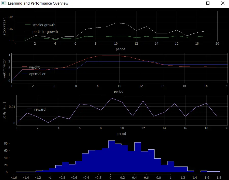
To illustrate the general idea of what we wanted to achive, below you can find a very naive graph which shows the convergence of an actor algorithm towards the analytically solved Merton Portfolio Lifecycle Problem. Each year (timeperiod of choice) the agend observes the market and makes a decision to invest some amount of wealth into stock, bonds or consumption. At the end of the period the agent gets rewarded. Thereby, the utility function acts as the reward that the agent receives for its investment decision. A good decision creates a good utility and vice versa. After enough training epochs the agent converges towards the optimal Merton solution and shows that it was able to perform optimal investment decisions maximizing its utility.